In this post I want to discuss an Internets phenomena knows as bots, specifically Twitter bots. I’m focusing on Twitter bots primarily because they’re fun and funny, but also because Twitter happens to provide a rich and comprehensive API that allows users to access information about the platform and how it’s used. In short, it makes for a compelling demonstration of Python’s prowess for data analysis work, and also areas of relative weakness.

For those unfamiliar with Twitter (who are you monsters?), it’s a social media platform on which users can post 140 character fart jokes called “tweets” (that joke bombed at PyData btw, but I can’t let it go). Twitter is distinct from other social media in that by default tweets are public and there’s no expectation that followers actually know one another. You can think of Twitter less as a stream of personal news, and more as a marketplace of ideas where the currency is favs and retweets.

After my death I'd like my remains to be vaped by everyone in my dance crew except for Li'l Sherbet. He knows why

— Andy Richter (@AndyRichter) July 31, 2015

Another distinguishing feature of Twitter is the “embed-ability” of its content (hilarious example above). It’s commonplace nowadays to see tweets included as part of news media. This is due in no small part to the openness of their APIs, which allow developers to programmatically tweet and view timelines. But the same openness that makes twitter pervasive across the internet, also opens the door for unwelcome users, like bots.

Twitter bots are programs that compose and post tweets without human intervention, and they range widely in complexity. Some are relatively inert, living mostly to follow people and fav things, while others use sophisticated algorithms to create, at times, very convincing speech. All bots can be a nuisance because their participation in the Twittersphere undermines the credibility of Twitter’s analytics and marketing attribution, and ultimately their bottom line.

So what can Twitter do about them? Well, the first step is to identify them. Here’s how I did it.

Creating labels

The objective is to build a classifier to identify accounts likely belonging to bots, and I took a supervised learning approach. “Supervised” means we need labeled data, i.e. we need to know at the outset which accounts belong to bots and which belong to humans. In past work this thankless task had been accomplished through the use (and abuse) of grad students. For example, Jajodia et al manually inspected accounts and applied a Twitter version of the Turing test–if it looks like a bot, and tweets like a bot, then it’s a bot. The trouble is, I’m not a grad student anymore and my time has value (that joke killed). I solved this problem thanks to a hot tip from friend and co-worker Jim Vallandingham, who introduced me to fiverr, a website offering dubious services for $5.

Five dollars and 24 hours later, I had 5,500 new followers. Since I knew who followed me prior to the bot swarm, I could positively identify them as humans and all my overnight followers as bots.

Creating features

Due to the richness of the Twitter REST API, creating the feature set required significantly less terms-of-service-violating behavior. I used the python-twitter module to query two endpoints: GET users/lookup and GET statuses/user_timeline. The users/lookup endpoint returns a JSON blob containing information you could expect to find on a user’s profile page, e.g. indicators of whether they’re using default profile settings, follower/following counts, and tweet count. From GET/user_time I grabbed the last 200 tweets of everyone in my dataset.

The trouble is, Twitter isn’t going to let you just roll in and request all the data you want. They enforce rate limits on the API, which means you’re going to have to take a little cat nap in between requests. I accomplished this in part with the charming method, blow_chunks:

# don’t exceed API limits
def blow_chunks(self, data, max_chunk_size):
  for i in range(0, len(data), max_chunk_size):
    yield data[i:i + max_chunk_size]

blow_chunks takes as input a list of your queries, for example user ids, and breaks it into chunks of a maximum size. But it doesn’t return those chunks, it returns a generator, which can be used thusly:

if len(user_ids) > max_query_size:
  chunks = self.blow_chunks(user_ids, max_chunk_size = max_query_size)
  while True:
    try:
      current_chunk = chunks.next()
      for user in current_chunk:
        try:
          user_data = self.api.GetUser(user_id = str(user))
          results.append(user_data.AsDict())
        except:
          print "got a twitter error! D:"
          pass
      print "nap time. ZzZzZzzzzz..."
      time.sleep(60 * 16)
      continue
    except StopIteration:
      break

If the query size is bigger than the maximum allowed, then break it into chunks. Call the .next() method of generators to grab the first chunk and send that request to the API. Then grab a beer because, there’s 16 minutes until the next request is sent. When there aren’t anymore chunks left, the generator will throw a StopIteration and break out of the loop.

These bots are weird

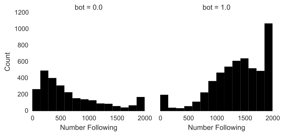
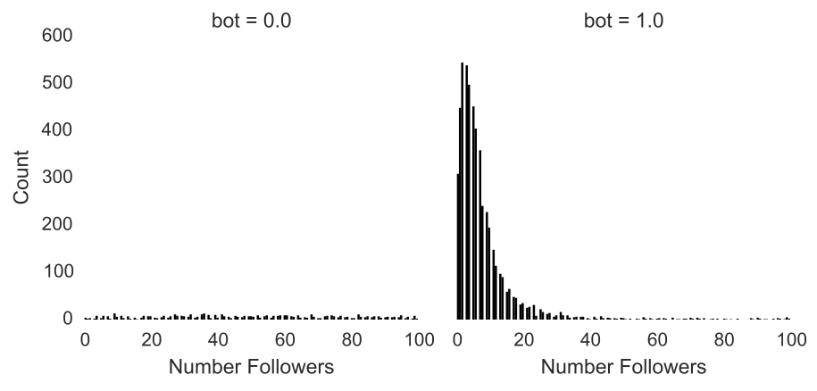
Fast-forward to clean, well-formatted data and it doesn’t take long to find fishiness. On average, bots follow 1400 people whereas humans follow 500. Bots are similarly strange in their distribution of followers. Humans have a fairly uniform distribution of followers. Some people are popular, some not so much, and many in between. Conversely, these bots are extremely unpopular with an average of a measly 28 followers.

Tweets into data

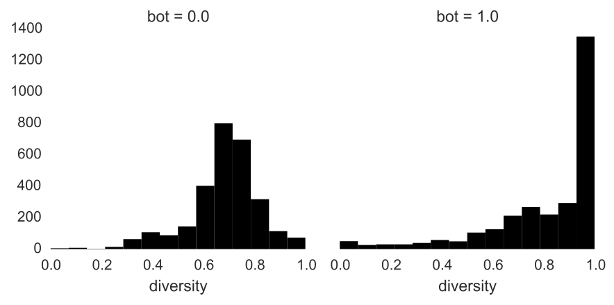
Sure, these bots look weird at the profile level, but lots of humans are unpopular and have the Twitter egg for a profile picture. How about what they’re saying? To incorporate the tweet data in the classifier, it needed to be summarized into one row per account. One such summary metric is lexical diversity, which is the ratio of unique tokens to total tokens in a document. Lexical diversity ranges from 0 to 1 where 0 indicates no words in a document, and 1 indicates that each word was used exactly once. You can think of it as a measure of lexical sophistication.

I used Pandas to quickly and elegantly apply summary functions like lexical diversity to the tweets. First I combined all the tweets per user into one document and tokenized it, so I was left with a list of words. Then I removed punctuation and stopwords with NLTK.

Pandas makes it super simple to apply custom functions over groups of data. With groupby I grouped the tweets by screen name and then applied the lexical diversity function to my groups of tweets. I love the simplicity and flexibility of this syntax, which makes it a breeze to group over any category and apply custom summary functions. For example, I could group by location or predicted gender, and compute the lexical diversity of all those slices just by modifying the grouping variable.

def lexical_diversity(text):
  if len(text) == 0:
    diversity = 0
  else: 
   diversity = float(len(set(text))) / len(text)
  return diversity
  
# Easily compute summaries for each user!
grouped = tweets.groupby('screen_name')
diversity = grouped.apply(lexical_diversity)

Again these bots look strange. Humans have a beautiful, almost textbook normal distribution of diversities centered at 0.70. Bots on the other hand have more mass at the extremes, especially towards one. A lexical diversity of one means that every word in the document is unique, implying that bots are either not tweeting much, or are tweeting random strings of text.

Model Development

I used scikit-learn, the premier machine learning module in Python, for model development and validation. My analysis plan went something like this: since I’m primarily interested in predictive accuracy, why not just try a couple classification methods and see which one performs the best. One of the strengths of scikit-learn is a clean and consistent API for constructing models and pipelines that makes trying out a couple models simple.

# Naive Bayes
bayes = GaussianNB().fit(train[features], y)
bayes_predict = bayes.predict(test[features])

# Logistic regression
logistic = LogisticRegression().fit(train[features], y)
logistic_predict = logistic.predict(test[features])

# Random Forest
rf = RandomForestClassifier().fit(train[features], y)
rf_predict = rf.predict(test[features])

I fit three classifiers, a naive Bayes, logistic regression and random forest classifier. You can see that the syntax for each classification method is identical. In the first line I’m fitting the classifier, providing the features from the training set and the labels, y. Then it’s simple to generate predictions from the model fit by passing in the features from the test set and view accuracy measures from the classification report.

# Classification Metrics
print(metrics.classification_report(test.bot, bayes_predict))
print(metrics.classification_report(test.bot, logistic_predict))
print(metrics.classification_report(test.bot, rf_predict))

Not surprisingly random forest performed the best with an overall precision of 0.90 versus 0.84 for Naive Bayes and 0.87 for logistic regression. Amazingly with an out-of-the-box classifier, we are able to correctly identify bots 90% of the time, but can we do better? Yes, yes we can. It’s actually really easy to tune classifiers using GridSearchCV. GridSearchCV takes a classification method and a grid of parameter settings to explore. The “grid” is just a dictionary keyed off of the model’s configurable parameters. What’s rad about GridSearchCV is that you can treat it just like the classification methods we saw previously. That is, we can use .fit() and .predict().

# construct parameter grid
param_grid = {'max_depth': [1, 3, 6, 9, 12, 15, None],
              'max_features': [1, 3, 6, 9, 12],
              'min_samples_split': [1, 3, 6, 9, 12, 15],
              'min_samples_leaf': [1, 3, 6, 9, 12, 15],
              'bootstrap': [True, False],
              'criterion': ['gini', 'entropy']}

# fit best classifier
grid_search = GridSearchCV(RandomForestClassifier(), param_grid = param_grid).fit(train[features], y)

# assess predictive accuracy
predict = grid_search.predict(test[features])
print(metrics.classification_report(test.bot, predict))

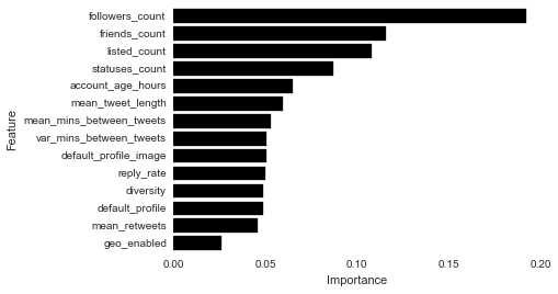
Aha, better precision! The simple tuning step resulted in a configuration that yielded a 2% increase in precision. Inspecting the variable importance plot for the tuned random forest yields few surprises. The number of friends and followers are the most important variables for predicting bot-status.

Still, we need better tools for iterative model development

There’s still a lot of room for growth in scikit-learn, particularly in functions for generating model diagnostics and utilities for model comparison. As an illustrative example of what I mean, I want to take you away to another world where the language isn’t Python, it’s R. And there’s no scikit-learn, there’s only caret. Let me show you some of the strengths of caret that could be replicated in scikit-learn.

Below is the output from the confusionMatrix function, the conceptual equivalent of scikit-learn‘s classification_report. What you’ll notice about the output of confusionMatrix is the depth of accuracy reporting. There’s the confusion matrix and lots of accuracy measures that use the confusion matrix as input. Most of the time you’ll probably only use one or two of the measures, but it’s nice to have them all available so that you can use what works best in your situation without having to write extra code.

> confusionMatrix(logistic_predictions, test$bot)
Confusion Matrix and Statistics

          Reference
Prediction   0   1
         0 394  22
         1 144  70
                                          
               Accuracy : 0.7365          
                 95% CI : (0.7003, 0.7705)
    No Information Rate : 0.854           
    P-Value [Acc > NIR] : 1               
                                          
                  Kappa : 0.3183          
 Mcnemars Test P-Value : <2e-16          
                                          
            Sensitivity : 0.7323          
            Specificity : 0.7609          
         Pos Pred Value : 0.9471          
         Neg Pred Value : 0.3271          
             Prevalence : 0.8540          
         Detection Rate : 0.6254          
   Detection Prevalence : 0.6603          
      Balanced Accuracy : 0.7466          
                                          
       'Positive' Class : 0 

One of the biggest strengths of caret is the ability to extract inferential model diagnostics, something that’s virtually impossible to do with scikit-learn. When fitting a regression method for example, you’ll naturally want to view coefficients, test statistics, p-values and goodness-of-fit metrics. Even if you’re only interested in predictive accuracy, there’s value to understanding what the model is actually saying and knowing whether the assumptions of the method are met. To replicate this type of output in Python would require refitting the model in something like statsmodels, which makes the model development process wasteful and tedious.

summary(logistic_model)

Call:
NULL

Deviance Residuals: 
    Min       1Q   Median       3Q      Max  
-1.2620  -0.6323  -0.4834  -0.0610   6.0228  

Coefficients:
                Estimate Std. Error z value Pr(>|z|)    
(Intercept)      -5.7136     0.7293  -7.835 4.71e-15 ***
statuses_count   -2.4120     0.5026  -4.799 1.59e-06 ***
friends_count    30.8238     3.2536   9.474  < 2e-16 ***
followers_count -69.4496    10.7190  -6.479 9.22e-11 ***
---

(Dispersion parameter for binomial family taken to be 1)

    Null deviance: 2172.3  on 2521  degrees of freedom
Residual deviance: 1858.3  on 2518  degrees of freedom
AIC: 1866.3

Number of Fisher Scoring iterations: 13

But I think the best feature of R’s caret package is the ease with which you can compare models. Using the resamples function I can quickly generate visualizations to compare model performance on metrics of my choosing. These type of utility functions are super useful during model development, but also in communication of early results where you don’t want to spend a ton of time making finalized figures.

# compare models
results = resamples(list(tree_model = tree_model, 
                         bagged_model = bagged_model,
                         boost_model = boost_model))
# plot results
dotplot(results)

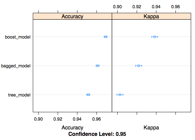
For me, these features make all the difference and are a huge part of why R is still my preferred language for model development.

Conclusion

If you learned anything from this read, I hope it’s that Python is an extremely powerful tool for data tasks. We were able to retrieve data through an API, clean and process the data, develop, and test a classifier all with Python. We’ve also seen that there’s room for improvement. Utilities for fast, iterative model development are rich in R’s caret package, and caret serves as a great model for future development in scikit-learn.